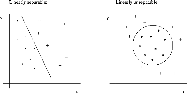
Since classification is usually the main problem in ESs, we will
concentrate on classification by neural networks and support vectore
machines (SVM). The main division of classifiers is to linear and
nonlinear. A linear classifier can separate two classes only,
when they are linearly separable, i.e. there exists a
hyperplane (in two-dimensional case just a straight line) that
separates the data points in both classes. An opposite case is that
classes are linearly inseparable. In this case it is still
possible that only few data points are in the wrong side of a
hyperplane, and thus the error in assuming a linear boundary is
small. Depending on the degree of error, linear classifier can still
be preferable, because the resulting model is simpler and thus less
sensitive for overfitting (poor generalization ability to new data
points). However, some classes can be separated only by a non-linear
boundary and we need a nonlinear classifier.

More precisly: Let's have numeric attributes X1,...,Xk, whose values are denoted by dom(Xi). For example if X1 can have values between 0<=X<=1, then dom(X1)=[0,1]. These compose attribute space dom(X1) x dom(X2) x ... x dom(Xk). All data points lie somewhere in this space. If the points fall into two classes, there is some boundary which separates them. If the classes are linearly separable, then in two-dimensional case we can describe the boundary by a line, for 3-dimensional data we need a plane and for higher dimensional data a hyperplane. One way to define this hyperplane is a discriminant function f(x1,..,xk), which is 0 on the plane, positive, when (x1,...,xk) belongs to class 1, and negative otherwise. The discriminant function is linear i.e. f=a1x1+a2x2+...+akxk+b.
The simplest example of non-linear boundary is exclusive-or function of two attributes: XOR(x1,x2)=1, if x1 is true or x2 is true, but not both. However, if we map the datapoints to higher dimensional attribute space, it becomes possible to separate the classes by a hyperplane.
Notice that Naive Bayes model using categorial data is linear classifier, while Naive Bayes with numeric data can recognize quite complex (nonlinear) decision boundaries. However, it is not as powerful as FFNN. Perceptron is an example of linear classifier. Decision tree does not recognize even linear boundaries, but the decision boundaries should be (piecewise) parallel to attribute axis. However, a complex decision tree can approximate even non-linear boundaries.
There is a large variety of neural networks, and we concentrate here only to the most commonly used model: feed-forward neural networks (FFNN). They can be seen as an enlargement of perceptrons (which were described in the slides; those containing just a layer of input nodes and another of output nodes) and sometimes FFNNs are called feed-forward multilayer perceptrons. A FFNN model consist of a layer of input nodes, a layer of output nodes and one or more hidden layers. All nodes in one layer are connected to all nodes in the following layer, and edges are assigned weights w. When a new data point x=(x1,x2,..,xk) is given to the model, each input node is given one attribute value xi, and the values are propagated ("fed") forward, until output nodes are reached and result can be read.
Learning a FFNN structure is usually implemented by backward- propagation algorithm. The basic idea is following:
The termination criterion can be e.g. a fixed number of cycles, or threshold for accepted error. Notice that we have to feed the same input points several times and learning can be very time consuming (the slower the more complex network structure we have). Another important observation is that the accuracy of resulting model is very dependent on initial parameters (structure, weights and termination criterion). Even with the same structure and input data we can learn a totally different model in the next trial. In practice, we have to try several network structures before the best one is found. Still the model may be only suboptimal (stuck into local optimum) or overfitted.
Despite of these problems, the FFNN neural networks have really large capacity: three-layer FFNNs are in principle able to represent any kind of regression or classification functions. As a contrast, the common perceptrons can represent only linear class boundaries. Naive Bayes classifiers (with numeric data) can also represent non-linear boundaries, but not all of them (i.e. they have weaker expressive power). However, it is good to remember that in practice, it is not always possible to learn an arbitrary 3-layer FFNN from the data and the resulting model can be highly overfitted.
Check a good article which discusses the sthregths and weaknesses of FFNNs: Duda: Learned from neural networks
The main idea of support vectors was very clearly explained in the slides for linearly separable case. Let's now study, how they manage in linearly nonseparable case.
SVMs use a very clever technique to find nonlinear boundaries for classes. The underlying idea is that when we map the data to higher dimension, then the classes become linearly separable and we can just search the hyperplane (with largest margin) like in linear case.
For example, when the actual class boundary is a circle x1^2 + x2^2 = 1 (in 2-dim), then the transformation phi(x)=(x1x2,x1^2, x2^2) produces a plane in 3-dimensional space.
However, the dimensionality of the new attribute space explodes rapidly, and it is not practical to compute this transformation actually. SVMs circumvent this problem by using kernel functions. Remember that it was enough to find support vectors, which define the largest margin ("thickest hyperplane"). So we actually need to know only the dot product of transformed support vectors u and v, i.e. phi(u)*phi(v). This can be evaluated by a suitable kernel function K(u,v)=phi(u)*phi(v) without even explicitely knowing phi! The only problem is to select the kernel function among several alternatives and often some knowledge about the domain is needed.
The main advantage of SVMs is that they find always the global optimum, because there are no local optima in maximizing the margin. Another benefit is that the margin does not depend on the dimensionality of data and the system is very robust for overfitting. Especially, when we have many attributes compared to number of rows, most of the other methods will fail. The model can be learnt in reasonable (quadratic) time for data sets of small and moderate size (hundreds of thousands data points). SVMs are flexible to handle different kind of modelling problems, although they are especially known for superior results in classification problem (compared to neural networks, for example). However, they have the same restriction than neural networks: the data should be continuous numerical. Categorial data can be handled, if it is first somehow coversed to numeric, but the results depend on how this conversation is done. The model is not very easily interpreted, and it can be hard for an expert to integrate her/his domain knowledge into model (in the form of kernel). And finally, we have the problem of selecting the parameters, although there are less parameters than in neural networks.
Question: It is claimed that a SVM model using a sigmoid kernel function is equivalent to a two-layer, feed-forward neural network. Can you find (or invent) the explanantion? I am interested to hear it!